Chapter 10 Effects
10.1 Types of effects from deploying the EDT
The Enterprise Digital Twin (EDT) delivers a combined effect across several levels: economic, managerial, strategic, and technological.
10.2 Economic effect
10.2.1 Direct cost savings
1. Lower operating costs (10–15%)
Sources of savings:
| Cost item | Savings | Mechanism |
|---|---|---|
| Raw materials and supplies | 5–8% | Procurement optimization, lower losses |
| Energy | 8–12% | Optimized equipment operating modes |
| Inventory | 15–25% | Optimized inventory levels |
| Logistics | 10–15% | Optimized routes and schedules |
| Downtime | 20–30% | Predictive maintenance, optimized schedules |
Sample calculation:
For an enterprise with annual operating costs of 10 billion rubles:
- Savings of 12% = 1.2 billion rubles per year
- Over 3 years = 3.6 billion rubles
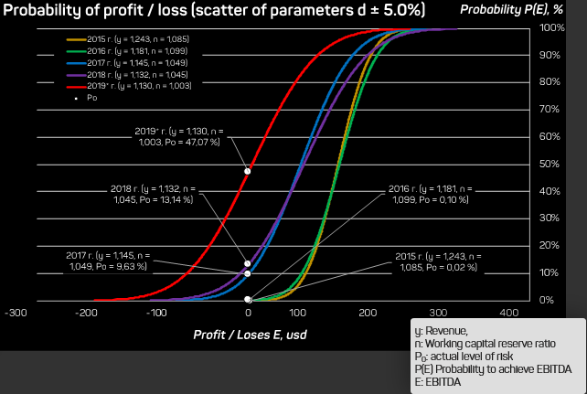
Figure 58 — Profit and loss probability: S-curves by year for assessing economic risk
2. Lower production cost (5–10%)
Drivers:
- Streamlined production processes
- Fewer losses and defects
- Higher energy efficiency
- Higher labor productivity
Impact on competitiveness:
- Room to cut prices by 3–5%
- Or to raise margins by 5–10%
- A larger market share
10.2.2 Higher revenue and profit
1. More output (10–20%)
Sources of growth:
- 15–20% higher equipment utilization
- 20–30% less downtime
- Optimized production cycles
- Better planning and capacity balancing
2. Higher product quality
Effects:
- 15–25% fewer defects
- Room to raise prices on premium products
- Higher customer satisfaction
- Repeat orders
3. New opportunities
Additional revenue:
- Launching new products (fast modeling)
- Customer-specific customization
- Handling more complex orders
- Premium prices for guaranteed quality
10.2.3 Working capital optimization
Freeing up funds:
Typical effect for an enterprise:
Starting figures:
- Raw material inventory: 500 million rubles
- Finished goods inventory: 300 million rubles
- Accounts receivable: 400 million rubles
- Total working capital: 1.2 billion rubles
After deploying the EDT:
- Raw material inventory: -20% = -100 million rubles
- Finished goods inventory: -25% = -75 million rubles
- Accounts receivable: -10% = -40 million rubles
- Freed up: 215 million rubles
Effect:
- Lower debt load
- Interest savings: 15–20 million rubles/year
- Capacity to invest in growth
10.2.4 Higher profitability
Combined effect:
Profitability = (Profit / Revenue) × 100%

Before deployment:
Revenue: 15 billion rubles
Costs: 13 billion rubles
Profit: 2 billion rubles
Profitability: 13.3%

After deployment:
Revenue: +15% = 17.25 billion rubles
Costs: -12% = 11.44 billion rubles
Profit: 5.81 billion rubles (+190%)
Profitability: 33.7% (+20.4 pp)10.3 Managerial effect
10.3.1 Faster decision-making
Time savings:
| Process | Before | After | Speedup |
|---|---|---|---|
| Production planning | 2–4 weeks | 1–2 days | 10–20x |
| Scenario analysis | 1–2 months | 2–3 days | 15–30x |
| Investment project appraisal | 2–3 weeks | 2–3 days | 5–7x |
| Cost calculation | 1–2 weeks | 1 hour | 80–160x |
| Demand forecast | 1 week | 2–3 hours | 15–30x |
Effect:
- Quick response to market shifts
- Room to weigh more options
- Better-grounded decisions
- Lower risk of errors
10.3.2 Better decision quality
Drivers of improvement:
1. Well-grounded decisions
- Decisions based on data, not intuition
- Quantified consequences
- Many factors taken into account
- Tested on the model before rollout
2. Lower risk
- Risks spotted early
- Quantified risks
- Mitigation measures
- Choosing the least risky options
3. Optimal decisions
- Finding the best option among many
- Balancing multiple goals
- Accounting for every constraint
- Surfacing non-obvious solutions
10.3.3 Management transparency
Process visibility:
For top management:
- The real state of the enterprise at any moment
- Tracking goal achievement
- Early problem detection
- Insight into trends and dynamics
For middle management:
- Real-time production status
- Inventory levels and utilization
- Unit productivity
- Plan-versus-actual analysis
For specialists:
- Detailed analytics across every process
- Access to historical data
- Analysis tools
- Room to test hypotheses
10.3.4 Coordination across units
A single information space:
- Every unit works from the same data
- Aligned plans
- Automatic synchronization
- Fewer conflicts
Effect:
- 50–70% less time spent on approvals
- 80% fewer errors from misalignment
- Better collaboration
10.3.5 Freeing up specialists’ time
Automating routine work:
Typical time split for an analyst:
Before deploying the EDT:
- Data collection: 40%
- Processing and reconciliation: 30%
- Analysis: 20%
- Producing recommendations: 10%
After deploying the EDT:
- Data collection: 5% (automated)
- Processing and reconciliation: 5% (automated)
- Analysis: 50%
- Producing recommendations: 40%
Result: focus on analysis and recommendations instead of routine work
10.4 Strategic effect
10.4.1 Competitive advantages
1. Speed of adaptation
- Quick response to market shifts
- Flexible production programs
- Staying ahead of competitors
2. Innovation
- Fast testing of new products
- Room to experiment without risk
- Digital prototyping
3. Reliability
- Guaranteed delivery on commitments
- Predictable results
- High product quality
10.4.2 Business scalability
Room to grow:
- Growth without a proportional rise in costs
- Easy to add new sites
- Wider geography
- A more diverse product portfolio
Effect:
- 20–30% revenue growth without adding staff
- Capacity to run a larger business
10.4.3 Resilience to crises
Crisis-response capabilities:
- Early threat detection
- Quick strategy adaptation
- Cost optimization without losing effectiveness
- Scenario planning
Examples:
- Quick adaptation to raw material price swings
- Retooling production when demand drops
- Optimization under resource constraints
10.5 Technological effect
10.5.1 Sample scenario modeling in agriculture
Using wheat production as an example, the system models scenarios for changes in production, consumption, and exports over a 2026–2030 horizon. Scenarios are set by changing external factors (population, consumption, the central bank rate, the dollar exchange rate, and others) and technological parameters, and the results appear as balance figures (thousand tons) and changes relative to the baseline scenario.
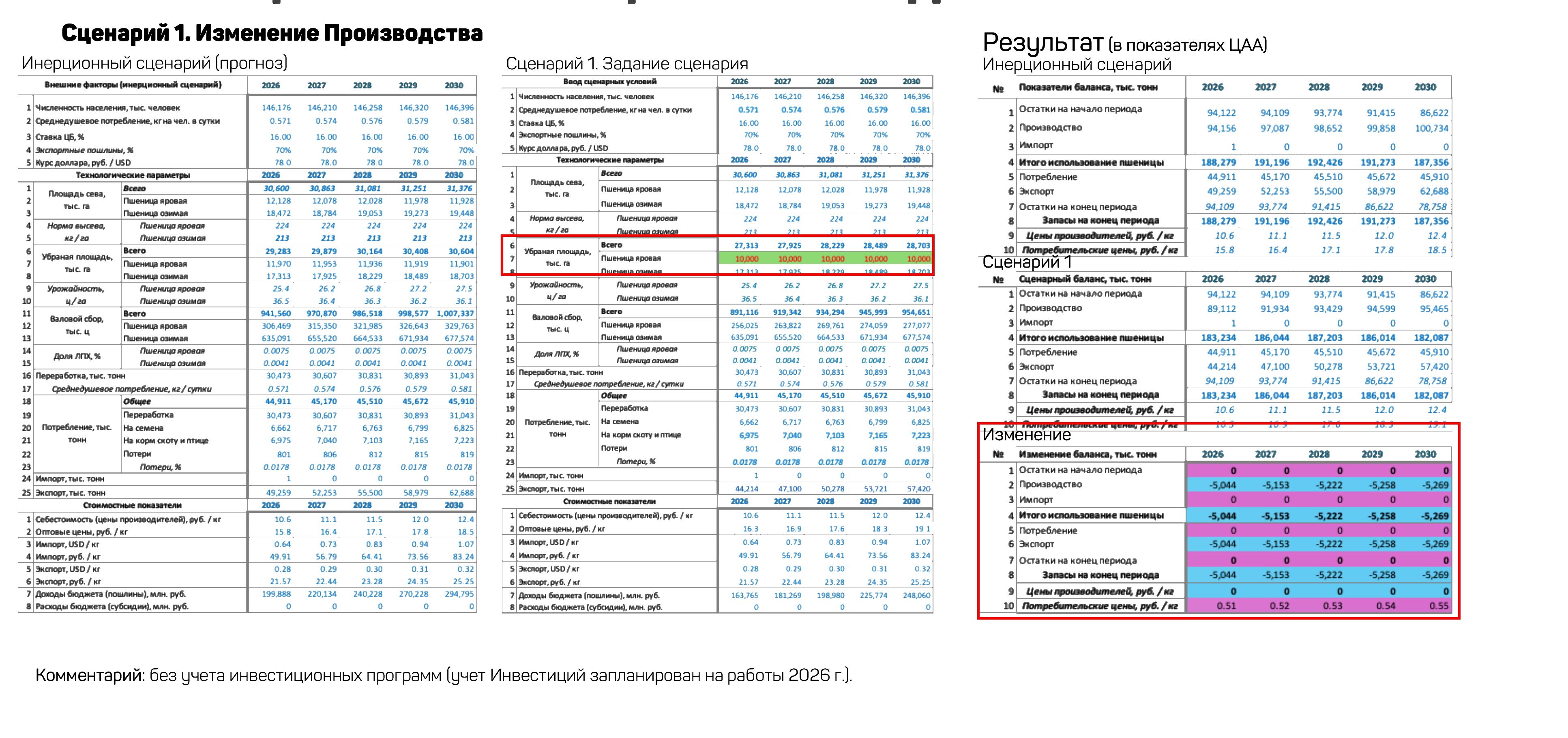
Figure 59 — Scenario modeling: a scenario for changes in wheat production with results in CAA metrics
10.5.2 Scale of the models built
For agriculture, the team built consumer price models for 134 products, 26 producer price models, 7 product balance models, proactive monitoring visualizations for executives, and a platform deployment on the customer’s side.
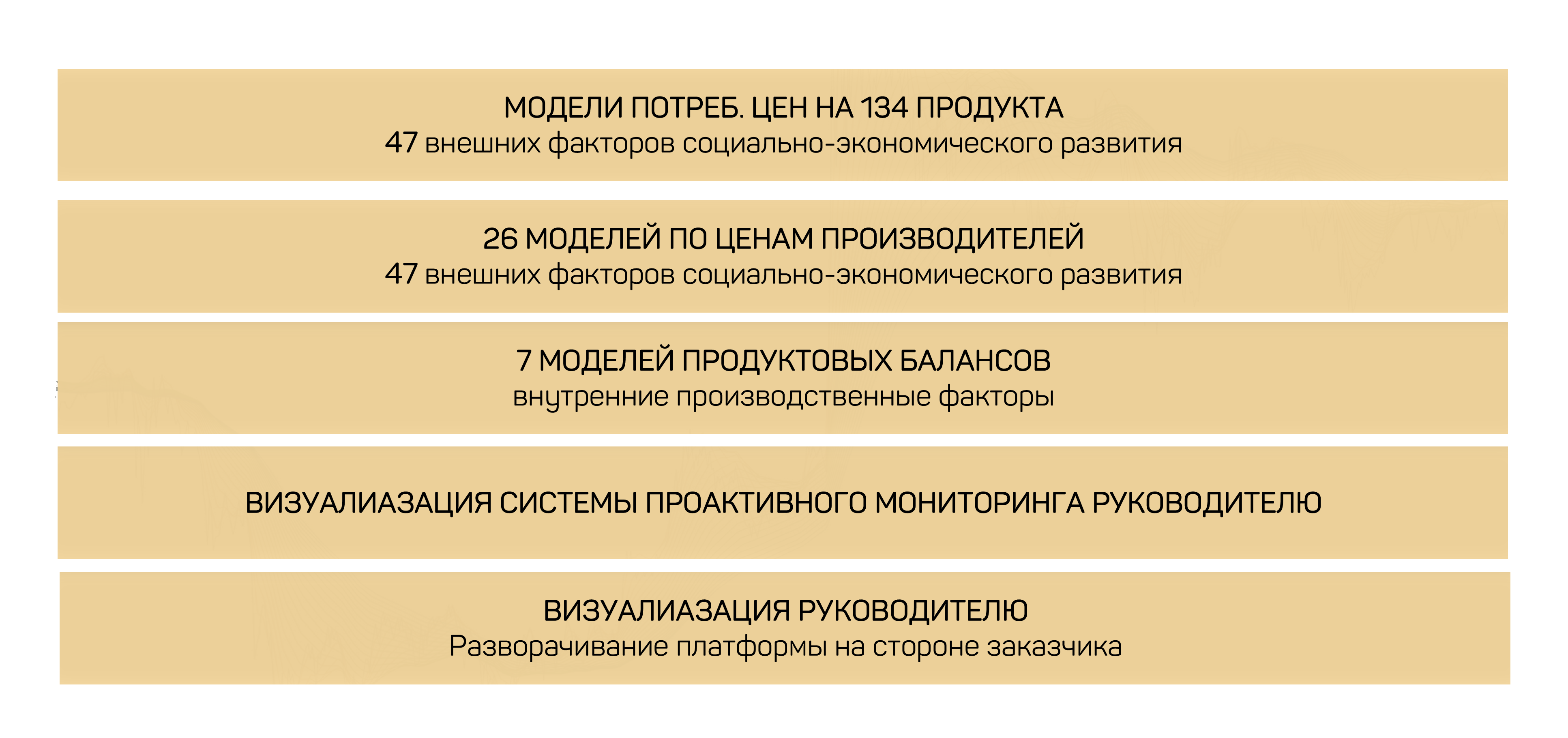
Figure 60 — Scale of the system built: 134 products, 26 models, 7 balances
10.5.3 Digital transformation
Steps toward Industry 4.0:
- Process automation
- A data-driven approach
- System integration
- Use of AI/ML
Result:
- A move to a new technological level
- Readiness for future challenges
- Attracting talent
10.6 Social effect
10.6.1 For employees
Better working conditions:
Skill development:
10.6.2 For society
Contribution to the economy:
10.6.3 Spatial mapping of metrics
Every metric carries an address, which makes it possible to rank and visually assess each territory’s share of the contribution (country, district, region, municipality). Color coding on the map reflects the risk level and helps quickly flag critical and stable territories.
Figure 61 — Spatial mapping of metrics: a multilevel map, color coding, rankings
10.6.4 Baseline forecasting and early warning
The calculated corridor reflects how stable a factor is over time and how accurate the model is, and it sets thresholds for early warning of an abnormal event. A break outside the corridor in the retrospective points to a possible error or distortion in the source data; as new factors appear, the baseline forecast recalculates across the entire system of metrics.
Figure 62 — Baseline forecasting of the metric system: the calculated corridor and early warning
10.6.5 Factor impact assessment
The system assesses each factor’s dynamic contribution to the risk level, how factors relate over time, projection onto the main factors, intersectoral, interterritorial, and agent-based effects, and ranks factors by how strongly they influence a chosen goal.
Figure 63 — Impact assessment: analyzing and assessing the root causes of price changes, ranking factors